This page assumes a working idea of how a neural network is trained; Mathematics for Machine Learning is a suitable refresher. Everything else is built from there.
Train a network, delete most of its weights and retrain what is left: it usually fails. The Lottery Ticket Hypothesis says that inside the original network there is a smaller subnetwork, a winning ticket, that trains on its own from its original random values to the accuracy of the whole network. The pruning leaves a mask that records which weights survive, and the random values the survivors started from are written θ0. What makes the claim unusual is that the exact initial values matter: swap them for fresh ones and the same subnetwork no longer recovers, as section 7 shows. The question this page answers is what finding a ticket costs, and whether the cheaper methods find one too.
1. The problem of over-parameterisation
Classical statistics says that test error follows a quadratic-like relationship with the number of parameters in a model, so that capacity beyond a certain point is harmful. Machine learning practice contradicts this. When the parameter count is raised far past that point, the model generalises well again, which is why networks are built with far more parameters than a task appears to need. This behaviour is the double descent phenomenon. As parameters are added, test error first falls, then rises to a peak where the model memorises the training set, and past that peak it falls a second time.
Test error falls, rises, and falls a second time. Classical statistics predicts the first descent and does not predict the second.
The left of the curve is the bias and variance trade-off. As capacity is added, test error falls, and then rises once the model begins to fit noise.
At the point where the model can fit the training set exactly, test error peaks. Classical statistics stops here and treats this capacity as excessive.
Past the peak, error falls again, and often below the classical minimum. Almost every model trained in modern machine learning relies on this second fall to generalise.
Most trained models sit in that second valley, on the far side of the peak. The accuracy is there, but every one of those parameters is still evaluated at inference.
If a network only needs a fraction of its weights to be accurate, can that fraction be found at a reasonable cost?
2. What the hypothesis claims
The hypothesis is stated in Frankle and Carbin's 2019 paper, The Lottery Ticket Hypothesis: Finding Sparse, Trainable Neural Networks. In one sentence:
A randomly-initialised dense network contains a subnetwork (a winning ticket) that, trained on its own from the same starting weights, matches the full network's accuracy in about the same number of steps.
A dense network can be treated as a book of lottery tickets, where each ticket is one of its 2n -1 possible subnetworks. Turning one over shows which connections it keeps.
Turning one over shows a dud: the subnetwork trains to an accuracy well below the full network's.
Training the dense network is therefore a search for the winning ticket.
Nothing about the winning ticket marks it out before training. The remainder of this page measures the work required to find it, and whether that work is worth doing.
The book is bigger than it sounds. The network this page trains has 797,184 prunable weights, so it contains about 10239,977 subnetworks — more than 10239,000 times the number of atoms in the observable universe. Every weight added doubles that count, and doubling the weights squares it. No method enumerates it; training the dense network is the only search that scales.
3. The dense network the experiment starts from
The experiment had to run on a laptop, so it uses MNIST and a network that is over-parameterised for that task. The network is fully connected, with no convolutions, to keep it simple. A flattened 28 by 28 image passes through three hidden layers and out to ten class scores.
class LargeMLP(nn.Module):
    def __init__(self):
        super().__init__()
        self.classifier = nn.Sequential(
            nn.Flatten(),
            nn.Linear(28 * 28, 512), nn.ReLU(),
            nn.Linear(512, 512),     nn.ReLU(),
            nn.Linear(512, 256),     nn.ReLU(),
            nn.Linear(256, 10),
)run_small_baseline.py over three seeds and reported as a mean.One neuron per pixel of a flattened 28 by 28 image.
784 into 512 is already 401,408 weights, more than half the network.
512, then 512, then 256 units. Every neuron connects to every neuron in the next layer.
Ten outputs, one for each digit from 0 to 9. About 797,000 weights in total, for a task on which the lean network on the right, with 31 times fewer weights, comes within a point.
All of these weights are trained. The rest of this page is about reducing the number that remain, so that inference costs less computation.
4. Ranking weights by magnitude
The simplest rule is magnitude pruning, and it performs well. The network is trained, every weight is ranked by its absolute value, and the smallest are removed. A weight whose magnitude has fallen close to zero contributes little to the output.
Most of the trained magnitudes sit near zero and contribute little to the output.
One round of pruning removes the smallest 20% by magnitude. Almost all of what it removes lies near zero, so the weights carrying signal are left in place.
A deeper cut reaches into the body of the distribution and reduces accuracy measurably. Section 5 shows why the cut is made in stages rather than in one step.
Pruning does not delete a tensor. Each layer carries a mask of ones for the weights that remain and zeros for those that have been pruned. All surviving weights are pooled, and a single global cutoff is taken from that pool.
def prune_by_magnitude(model, masks, prune_rate):
    # pool all still-alive weights, find the prune_rate-smallest by |w|
    all_weights = torch.cat([
        module.weight.data[masks[name] == 1].abs().view(-1)
        for name, module in model.named_modules() if name in masks
    ])
    k = int(prune_rate * all_weights.numel())
    threshold = torch.topk(all_weights, k, largest=False).values[-1]

    for name, module in model.named_modules():
        if name in masks:
            new_mask = torch.where(module.weight.data.abs() > threshold, 1.0, 0.0)
            masks[name] *= new_mask          # keep existing structural zeros
    return masks
A single cutoff for the whole network does not treat the layers equally. The large hidden layers hold most of the near-zero weights, so they are emptied far faster than the small output layer. Section 9 shows the consequence.
5. Iterative Magnitude Pruning and the rewind
Removing 90% of the weights in one step is possible, but doing so in stages performs considerably better. Iterative Magnitude Pruning repeats a short loop, removing about 20% of the remaining weights on each pass.
Step four is what distinguishes the lottery ticket method from ordinary pruning. After each round of cutting, the surviving weights are rewound to θ0, the values they held at initialisation, saved before a single gradient step was taken. They do not keep the values they learned, and they are not given fresh random values. The smaller network is then trained, pruned, rewound, and the loop repeats.
init_state = copy.deepcopy(model.state_dict())   # theta_0, saved BEFORE training
masks = convert_to_mask(model)

for iteration in range(1, pruning_iterations + 1):
    masks = prune_by_magnitude(model, masks, prune_rate)  # trim the smallest |w|
    model.load_state_dict(copy.deepcopy(init_state))      # rewind to theta_0
    apply_mask(model, masks)                              # re-impose the structure
    train(model, masks)                                   # retrain the subnetwork
One implementation detail matters here. The mask has to be reapplied after every optimiser step rather than once per round. An optimiser with momentum, such as Adam, will otherwise carry a pruned weight back off zero. Re-masking at every step holds the pruned weights at zero.
6. Does the method work?
This is the result the rest of the page depends on, taken from the cached run. The winning ticket is shrunk into extreme sparsity and its test accuracy is recorded at each round.
Blue holds the dense baseline as the network is cut down, and in places sits slightly above it. Most of the weights are removed and almost all of the accuracy is retained.
Orange keeps the winning ticket's exact masks and gives the survivors fresh random values. With the correct structure and the wrong initialisation, it never recovers the baseline.
Purple removes a random set of weights to the same sparsity and rewinds to θ0. With the correct initialisation and the wrong structure, it falls away fastest of the three.
Retaining accuracy while pruning is, on its own, evidence of good pruning but not really more. The question is why the accuracy holds, and answering it requires controls.
7. Why it is a ticket: the controls
The hypothesis depends on two conditions at once: the correct structure, which is the mask that magnitude pruning finds, and the correct starting point, which is θ0. To test whether both are required, the same pruning schedule is run twice more, with one of the two conditions broken in each run.
- Random re-initialisation. The winning ticket's exact masks are kept, and the survivors are given fresh random values in place of θ0. The structure is correct and the starting point is not.
- Random pruning. A random set of weights is removed to the same sparsity and the survivors are rewound to θ0. The starting point is correct and the structure is not.
Both controls fall away from the winning ticket as sparsity increases. Neither the structure alone nor the starting point alone accounts for the result; the two are required together.
The clearest evidence is in how fast the network learns. At a fixed high sparsity, the winning ticket reaches a higher final accuracy, and it also starts from a lower loss and falls faster than the same mask initialised at random.
The surviving connections are a winning ticket only together with the values they started from. Once those values are replaced, the ticket is lost.
8. What a winning ticket costs to find
The sections above establish that winning tickets exist. They do not establish that the tickets are worth what they cost. Iterative Magnitude Pruning produces a network that is cheap to deploy and expensive to find. The remainder of this page measures that cost.
The cost can be stated as a number. From this point on, the experiment trains for three epochs per round and prunes 20% of the survivors each round, out to 21 rounds. Reaching 99% sparsity in this way requires training the network 21 separate times, which is 63 epochs of training spent before a mask exists, on a network that reaches 97.7% accuracy in three. This is the cheaper variant of the method. In the original paper each round trains to convergence, so a faithful run costs considerably more, and the figure of 63 epochs is therefore a lower bound.
Search cost is defined here as the number of training epochs spent before a mask exists. Everything after that point is identical for every method: the survivors are rewound to θ0, trained for three epochs, and their test accuracy is measured.
Fixing the training budget after pruning is what makes the comparison valid. If one method were allowed to train for longer, it would win for a reason unrelated to the quality of its mask.
IMP decides last and pays the most, at one full training run per pruning round and 21 rounds to reach 99% sparsity.
One-shot pruning trains the network a single time and makes the whole cut in one pass. Early-bird cuts earlier still, a few epochs into training.
SNIP scores connections from the gradients of a single minibatch. SynFlow scores them without reading the data at all. Both cost zero training epochs. (These methods are discussed in more detail in section 9.)
The accuracies beside each marker are what that method's ticket reaches at this sparsity. The position on the axis predicts them poorly.
9. Deciding at initialisation
The most aggressive option is to prune before training begins. If the weights can be ranked by some score computed at initialisation, no search cost is paid at all. The question is whether any score computed at θ0 carries enough information to produce that ranking.
SNIP: which connections the loss depends on
SNIP attaches an indicator variable to every connection, switches them all on, and measures how much the loss would change if a single connection were switched off. That derivative is the saliency. It costs one forward and one backward pass on a single minibatch and takes no optimiser step. The paper defines the criterion as a derivative with respect to the indicator, not the weight, so it measures the effect of removing a connection rather than changing its value. By the chain rule this reduces to the weight gradient multiplied by the weight: one line of code.
def snip_scores(model, batch, criterion, device, masks=None):
    model.zero_grad(set_to_none=True)
    data, target = batch
    loss = criterion(model(data.to(device)), target.to(device))
    loss.backward()
    return {n: (m.weight.grad * m.weight.data).abs().detach()
            for n, m in _linear_layers(model).items()}
The gradient is multiplied by the weight, the absolute value is taken, and the result is ranked globally across the network. That is the whole method. It performs adequately, but it is not free: its cost appears in accuracy rather than in epochs. At 10.7% of weights remaining, SNIP reaches 96.96% against IMP's 98.25%, having spent no training epochs against IMP's 30. The 1.3-point gap does not close as pruning continues. At 0.92% remaining, SNIP reaches 91.16% and IMP reaches 96.76%. SNIP loses accuracy slowly, where the methods in the next two sections fall sharply.
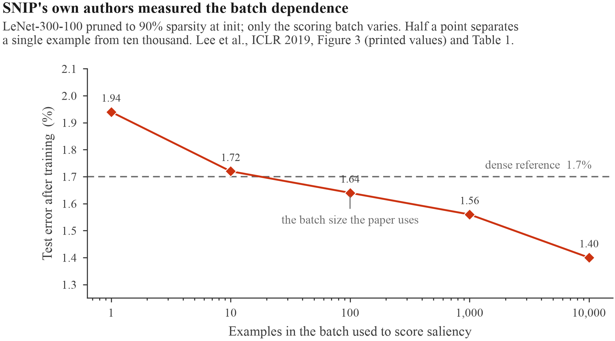
The effect of the sampled batch does not have to be estimated here, because the authors measured it. On a LeNet-300-100 pruned to 90% at initialisation, scoring the saliency on a single example gives 1.94% error after training, and scoring on ten thousand gives 1.40%, below the paper's own dense reference. Their batch-size sweep is drawn in the appendix.
Layer collapse, and what SynFlow does about it
A global saliency score has no reason to distribute its cuts evenly across layers. If one layer's scores are low as a group, a global threshold empties that layer first and continues until nothing remains in it. This is layer collapse: the algorithm prunes every parameter in one layer while prunable weights remain elsewhere. The network is then severed, and training cannot repair it, because no path remains from the input to the output.
Under a single global threshold, the large input layer loses weights fastest and the small output layer retains most of its own.
At 99.95% sparsity, SNIP has removed the last weight from the 784 to 512 layer. No signal can reach the output, so the network returns a constant for every input.
At the same sparsity, SynFlow still holds weights in all four layers. It collapses an order of magnitude later, at 99.99%, where about eighty weights remain in total.
The random mask is included as a reference. It thins every layer at the same rate, which neither saliency score does. Later sections return to this comparison.
SynFlow is constructed to avoid this, and it rests on two ideas. The first is the score itself. The absolute value of every parameter is taken, a single all-ones vector is passed through the network, and the outputs are summed. Every weight and activation is then non-negative, so that sum is the total signal flowing from the input to the output, and a weight's saliency is its share of that flow. The score reads no training example.
scorer.zero_grad(set_to_none=True)
ones = torch.ones((1, *input_shape), dtype=torch.double, device=device)
scorer(ones).sum().backward()          # R = total flow through the network
scores = {n: (m.weight.grad * m.weight.data).abs()
          for n, m in _linear_layers(scorer).items()}
The second idea explains why SynFlow does not collapse. The score is conserved: summed over any set of parameters that separates the input from the output, it always comes to the same value. Thinning a layer therefore raises the score of every weight remaining in it, so the layer protects itself. This holds only if the network is re-scored, which is why SynFlow is iterative, running a hundred rounds and cutting a little further on each. A hundred rounds appears expensive, but each round is one forward and one backward pass on a single input vector, and the procedure costs less than a tenth of one training epoch.
On this network, SynFlow and SNIP reach the same accuracy as each other: 96.95% against 96.96% at 10.7% remaining, and 91.21% against 91.16% at 0.92% remaining. A spread check was run by retraining fixed masks with only the data ordering changed. Single numbers move by 0.2 to 0.7 points under that change, which is larger than either gap.
SynFlow's theorem concerns trainability: the algorithm can compress down to one parameter per layer without disconnecting the network. Whether a network that thin is accurate is a separate question, and on this network it is not. SynFlow also collapses in this run, at 99.99% sparsity. The schedule used here runs for a fixed hundred rounds, and a longer schedule may hold the last layer open further. That was not tested.
10. Deciding a few epochs in
If pruning at θ0 is too early and pruning after full training is too expensive, the question is how early is early enough. The early-bird paper makes this answerable through one observation: the mask stops moving long before the network stops learning. The magnitude mask is computed after each epoch, its distance from the previous epoch's mask is measured, and the cut is made once those distances become small.
The published version does this with channel masks read from batch-norm scaling factors. The network used here has no convolutions and no batch norm, so the same idea is applied to unstructured weight masks instead. This is a substantial deviation from the published method. Their stopping rule is kept, along with their queue length of five and their threshold of 0.1, but these are applied to a mask over 797,184 weights rather than over a few thousand channels. A threshold of 0.1 on a mask of that size is a much weaker test, and the results below reflect that.
At 99% sparsity, half of the surviving structure is replaced between the first two epochs, and by epoch twenty about a quarter of it is still being replaced each epoch.
Measured the paper's way, as a fraction of all weights rather than of the survivors, the distances are small by construction: 5.7% at epoch two, falling to 2.9%. Both are already below the threshold, so the rule fires at epoch six for almost every sparsity level, which is the earliest that a queue of five consecutive distances permits. The rule is reporting the length of its own queue.
With the stopping rule removed, cutting after one epoch gives 97.82%, after five gives 98.45%, which is the highest value anywhere in this experiment, and after twenty gives 98.05%. IMP, having spent 30 epochs, reaches 98.25%.
Whatever property makes a mask good is fixed within an epoch or two. The changes after that point are among weights that appear to be interchangeable.
The mask therefore never converges, and it does not need to. Whatever property makes a mask good is fixed within an epoch or two, and the changes after that point are among weights that appear to be interchangeable. No satisfying explanation for this has been published.
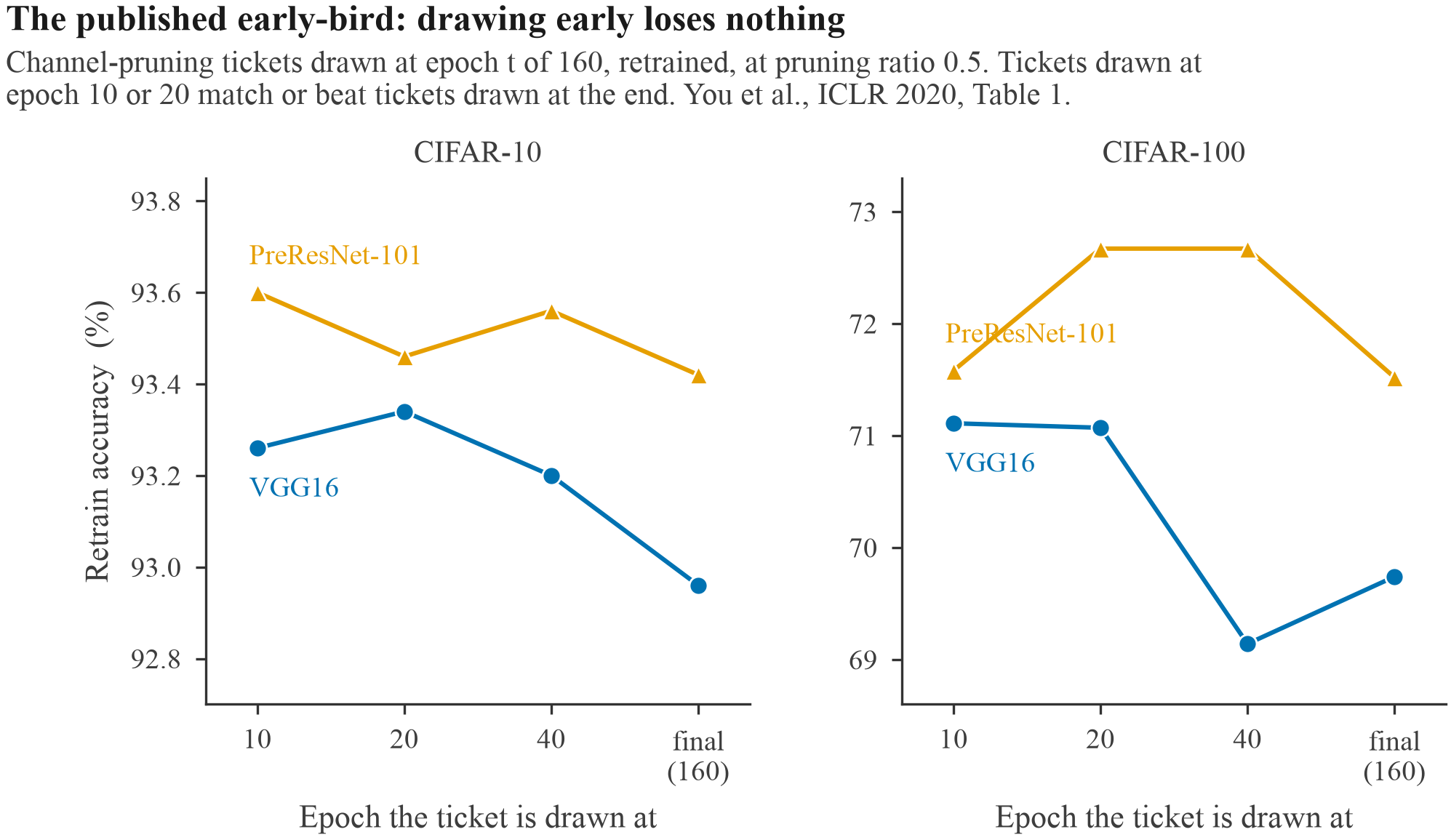
Because the variant used here is not the published method, the version to rely on is theirs. You et al. report it for the structured early-bird method: a channel-pruning ticket is drawn at epoch 10, 20, 40 or at the end of 160 epochs, retrained, and compared. On both networks and both datasets, the ticket drawn at epoch 10 or 20 matches or exceeds the ticket drawn at the end of training; their chart is in the appendix.
The limitation appears at extreme sparsity. At 0.92% of weights remaining, the early-bird ticket reaches 20.81%, against 97.7% for the dense network and 10% for guessing at random. It is the weakest method on this page at that point, and well behind cutting at random. Deciding early is adequate when nine weights in ten are removed. At 999 in 1000, six epochs of evidence is insufficient, and the per-layer budget inferred from it is wrong by enough to destroy the network.
11. Deciding once instead of twenty-one times
The final method is the simplest, and over most of the sparsity range it gives the best return on its cost. The network is trained once, the whole cut is made in a single pass, and the survivors are rewound and retrained. Frankle and Carbin compare this against iterating in their original paper and report the comparison as a curve rather than as a single number. That is the right form for the result, because the answer depends entirely on the sparsity at which you read it.
Blue reaches each sparsity through a sequence of prune, rewind and retrain rounds. Pink reaches the same sparsity from a single training run and one cut.
Down to about 5% of weights remaining, the two curves lie on top of each other. At 10.7% remaining, one-shot is ahead at 98.40% against 98.25%, for a tenth of the cost.
At 0.92% remaining, IMP holds 96.76% and one-shot falls to 66.49%. That is sixty-three epochs against three, for a difference of thirty accuracy points.
Iterating pays off only after a certain sparsity. Before that point it costs 63 epochs and changes almost nothing; after it, a single cut collapses. The only way to learn which side you are on is to test past the point.
Cheaper methods are safe while the network is only moderately sparse. Where that stops being true depends on the network and the schedule, and the only way to find the crossover is to train past it. That is what the 63 epochs of section 8 pay for.
12. Everything on one axis
The argument of this page comes down to one chart. Six ways of choosing the mask are plotted against what each one costs to find. The sparsity slider rearranges the ranking.
Three methods land within 0.15 points of each other, and the method that cost thirty epochs is not the highest of them. One-shot reached this point for three epochs, early-bird for six and IMP for thirty, and they are separated by less than the run-to-run variation.
SNIP and SynFlow sit below that cluster, level with each other, about 1.3 points back, and cost no training epochs. Below them is cutting at random, which is the weakest method here and the only one that uses no information about the network.
Past about 2% of weights remaining, the ordering rearranges completely. Early-bird fails first, followed by one-shot and then the random mask.
At the sparsest level, only IMP remains above 96%, and it is the only method that paid a substantial search cost. This is the single point in the sweep at which its sixty-three epochs return anything.
At mild sparsity, the long search is not worth performing. Training once and cutting once finishes level with the method that trains twenty-one times. The full curves show where that ceases to hold.
From the dense network on the left to under 1% of weights on the right. Over most of that range, every method lies within a couple of points of the others.
The three methods that train before they cut remain together down to about 5% remaining.
The two zero-cost scores sit a point or two below them across the whole range, and they decline gradually rather than failing.
Between 3% and 1% remaining, the methods separate, and the resulting order bears no relation to what each method cost.
13. No method recovers IMP's ticket
So the cheap methods match the expensive one over most of the sparsity range. That result leaves one question unanswered. When one-shot matches IMP's accuracy, is it finding the same subnetwork?
It is not. The two masks overlap far less than their matching accuracies suggest.
The dashed line is the overlap that two unrelated masks of that density reach by chance, which is the only defensible zero point. The random mask sits on it, which confirms that the measure behaves as expected.
At 10.7% remaining, the highest agreement anywhere is one-shot at 0.218, and one-shot starts from the same trained weights as IMP. SNIP reaches 0.124 against a chance level of 0.057.
By 0.92% remaining, every value is in single-digit percentages: SNIP 0.041, SynFlow 0.033 and one-shot 0.027. These masks are not the same as each other, yet their accuracies match.
Dividing through by the chance floor raises the values, though not by much. Exceeding chance by a factor of two is a weaker claim than recovering what IMP found.
A winning ticket is therefore not one specific set of weights that a method either finds or misses. What the scores contribute has a published answer.
Frankle, Dziugaite, Roy and Carbin ran an ablation on every pruning-at-initialisation method available to them. The mask is permuted within each layer, so that every layer keeps exactly the number of weights the method assigned to it while the choice of which weights is randomised. If a method identified the individual connections that matter, this ablation would destroy its result. It does not. Their conclusion, in their words, is that the useful information these techniques extract is not which individual weights to remove, but the layerwise proportions by which to prune the network.
Shuffling SynFlow's mask inside each layer costs between 0.1 and 0.8 points at every sparsity from 80% remaining down to 0.92%. SNIP loses about a point through the middle of the range and nothing at the sparse end.
A uniformly random mask has no per-layer budget beyond what uniform sampling produces, and it keeps the same number of weights overall. At 0.92% remaining, SynFlow's shuffled mask reaches 91.01% and the uniform random mask reaches 60.21%.
That gap comes entirely from how the survivors are divided between layers, since the choice of individual weights is randomised in both cases. SynFlow is computing a per-layer capacity allocation, in under a second and without reading the data, rather than identifying important weights.
When the difference is plotted directly, both lines sit on zero across the whole range. That flatness is the finding. Whatever information the score carries, it is not which connections to keep.
14. What happens at budgets this experiment cannot run
Every result above comes from one fully connected network on MNIST, run on a laptop. Frankle, Dziugaite, Roy and Carbin's 2021 paper reports on that same setting, a LeNet-300-100 on MNIST, and finds "little distinction between the performance of magnitude pruning after training and the early pruning methods—just a small fraction of a percent". They state this to make the point that MNIST is unrepresentative.
That criticism is correct, and its size is worth establishing. What follows is other authors' numbers, at scales this experiment cannot reach, selected so that the same methods sit on the same grid.
- At moderate sparsity, do not pay for IMP. One-shot and early-bird match it for a tenth to a fifth of its search cost (3 and 6 epochs against 30), and the gaps between them are inside the run-to-run variation (section 12).
- Past the crossover, nothing cheap survives. At 0.92% of weights remaining on this network, one-shot falls to 66.5% and early-bird to 20.8%, against IMP's 96.8%.
- At scale, rewind to an early checkpoint θk, not θ0. On ResNet-50, rewinding all the way to initialisation reaches 73.7% against a dense 76.1% and barely beats random pruning at 73.1%. Rewinding to about epoch 5 of 90 is the fix.
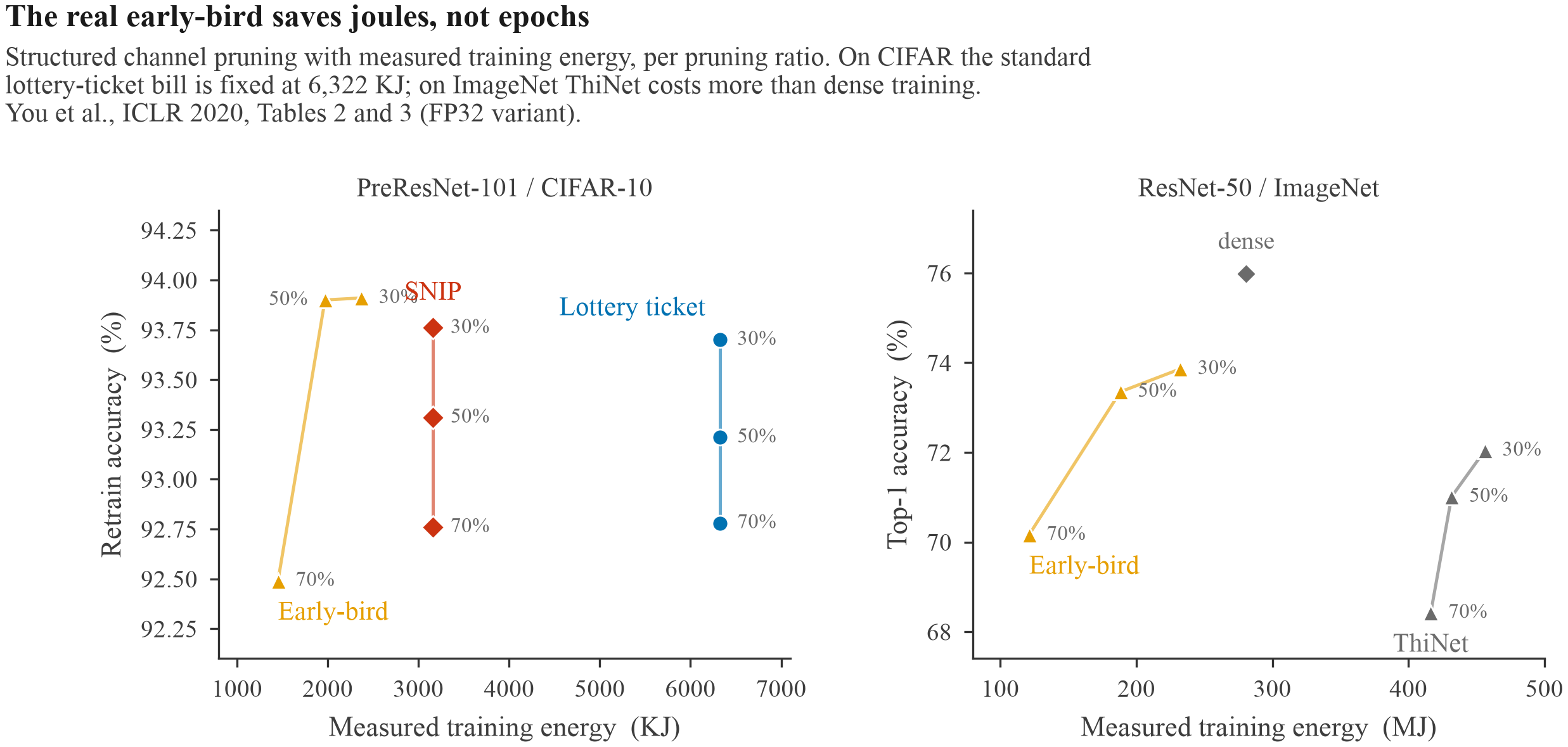
- Count joules, not epochs. On CIFAR-10 the standard lottery-ticket pipeline costs 6,322 KJ at every pruning ratio; the structured early-bird matches its accuracy at 30% and 50% pruning for 23–38% of that energy.
- Check saliency scores at scale before trusting them. On ImageNet at 94.5% sparsity, SNIP scores 46.0% while pruning at random scores 59.1%, so a score can be worse than no score at all.
- Sparsity on paper is not speed. An unstructured mask cuts parameter count; wall-clock and energy savings come from structured methods, and the joule measurements are of exactly those.
Every number behind those bullets, with the full tables and the published figures, is in the appendix. What follows here is the one correction that the experiment on this page cannot detect, and the four findings scored against the published work.
The same grid at the sparsest point each paper swept is in the appendix, and it carries the strongest published result of this comparison. On ImageNet at 94.5% sparsity, SNIP reaches 46.0% and pruning at random reaches 59.1%, so the saliency score is thirteen points below using no score at all. SynFlow, on the same network at the same sparsity, reaches 62.4%. The two methods that section 9 treats as interchangeable are therefore 16.4 points apart. This could not have been observed on MNIST at any sparsity tested here.
The shuffle result holds at scale
Section 13 contains the one finding from this experiment that can be defended at scale, because the same ablation was run there: shuffling raises accuracy in eleven of the sixteen cells and costs at most 0.7 points in the rest, and the grid, which includes ImageNet, is in the appendix. Two qualifications apply. The paper prints one counterexample it does not discuss: shuffled SNIP on ResNet-50 at 94.5% sparsity falls to 0.1%, which on a thousand classes is chance. And the thirty-one-point figure measured here for destroying the per-layer budget is larger than any comparable published figure; the nearest analogue, replacing the initialisation with a standard normal so the variance scaling behind magnitude pruning's layer budget is lost, costs 0.8 points on ResNet-20, 3.5 on VGG-16 and 9.7 on ResNet-18. The direction of the effect agrees and the size does not, by roughly a factor of three.
The cost of these methods, as reported
The ledger of reported costs, in which no two rows share the same units, is in the appendix. Its most informative line is the last one: the authors with the compute to run this comparison properly still ran out of it, and the cells they could not afford are the ones that would have tested their headline claim at scale. None of these papers reports GPU-hours, wall-clock time or expenditure for any experiment, so measured energy is the one axis that compares across papers, and the appendix carries that figure.
The correction that this setup cannot detect
One published result undermines the protocol used throughout this page. Rewinding to θ0 works on MNIST and does not work on larger networks. An IMP subnetwork of ResNet-50 rewound to initialisation reaches 73.7% against a dense 76.1%, while random pruning reaches 73.1% and random reinitialisation reaches 73.4%. At that scale the winning ticket does not exceed its own controls.
The correction is to rewind later. The relevant measure is stability: whether two copies of the network, trained onward with different data ordering, can be joined by a straight path along which the error does not rise. IMP subnetworks reach that point early, at iteration 500 of 63,000 on ResNet-20 and at epoch 5 of 90 on ResNet-50, and the rewind points at which subnetworks become matching coincide closely with the points at which they become stable.
This parallels section 10, where the mask settles enough to cut after about one epoch and no satisfying explanation has been published. Their result concerns the weights, which reach a stable basin after about five epochs out of ninety, and that stability is what makes rewinding work. These are different measurements, but both say the useful information about a subnetwork appears within the first few percent of training.
The four findings of this experiment, assessed against the published work
- One-shot matches iterative down to about 5% remaining. The original paper prints one-shot tickets on MNIST exceeding the dense network down to 5.17% remaining, and the crossover measured here fell at about 5%. That agreement was a coincidence that was not engineered: their comparison is one-shot against dense, not against iterative. No paper prints where one-shot stops matching iterative at any scale above MNIST, so this crossover is unreplicated rather than contradicted.
- Early-bird fails hardest at extreme sparsity. No published data exists either way, and the variant used here is not the published method. Their experiments do not test above 70% channel pruning, so the regime described here has not been measured elsewhere.
- SNIP and SynFlow are indistinguishable, 1.3 points behind IMP. This is half wrong. The tie holds at matching sparsity and breaks by 16.4 points at ImageNet extremes, and the 1.3-point gap is an artefact of MNIST that becomes 6.9 points on TinyImageNet.
- Shuffling costs nothing and the per-layer budget decides the result. This agrees with the published work, and it is the strongest of the four findings, because it replicates on ImageNet and because the paper closes the obvious confound: at the highest matching sparsity the shuffled network is at most 1.0026× as effectively sparse as the unmodified one (0.05% in most cases).
Three of the four findings are therefore properties of MNIST. The fourth is a property of pruning.
15. What this does and does not show
The caveats carry more weight than usual here, because a single small experiment of this kind readily produces a confident conclusion that is wrong.
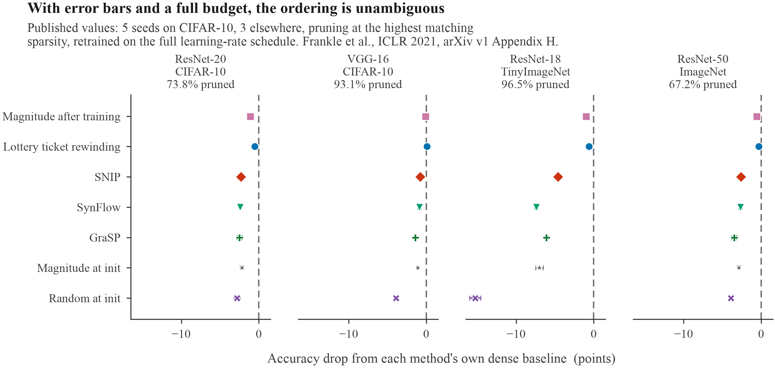
- One network, one dataset, one seed. To establish what a single number is worth, fixed masks were retrained with only the data ordering changed. Accuracies move by 0.2 to 0.7 points at both sparsities tested, and by up to 3 points for the random mask at extreme sparsity. Any gap below half a point should therefore be read as zero. The published grid in the appendix is this comparison run properly, over 3 to 5 seeds and four networks, and its error bars are smaller than every gap it reports.
- SNIP's score depends on which minibatch it is given. Two runs differing only in the sampled batch gave 96.96% and a mean of 97.29% at the same sparsity. That variation is a property of the method rather than of this implementation, and the authors' own batch-size sweep in section 9 bounds it at half a point between scoring on one example and on ten thousand.
- The training budget after pruning is three epochs, which is short. Any method that produces a subnetwork which learns quickly is favoured by that budget. The published grid in the appendix retrains on the full learning-rate schedule and the ordering holds there, so the short budget is not what places the at-init scores behind, although it could still reorder the middle of these results.
- The early-bird variant used here is not the published early-bird. The published method prunes channels using batch-norm scaling factors under an L1 penalty, and the energy savings it reports follow from that structure. The variant used here is unstructured, so it inherits the idea and none of the hardware benefit. Sections 10 and 14 carry the published version's own numbers: drawing at epoch 10 of 160 costs no accuracy, and the measured energy savings hold.
- Search cost measured in epochs ignores wall-clock time by design. On real hardware, SynFlow's hundred scoring passes are close to free and IMP's 63 epochs are not, so the epoch axis favours IMP. The energy figure in the appendix is the corrected axis: in measured joules, the standard lottery-ticket pipeline costs about four times what the published early-bird costs at 70% channel pruning.
- Sparsity on paper is not sparsity on the clock. Nothing here makes a network faster. It reduces the parameter count, which is a separate property. The nearest published numbers confirm this rather than resolve it. Renda et al.'s 4.8x speedup for learning-rate rewinding against 1.7x for fine-tuning on ResNet-50 is a theoretical FLOP count, and the joules measured by You et al. come from structured channels. An unstructured mask reduces parameter count and not time.
- The appendix tables are other authors' numbers, so they inherit other authors' problems. Their protocols differ from the protocol used here and from each other, several report no error bars, and one discloses a bug that tripled the learning rate for every model it trained. Only values printed as text have been quoted, and a printed value is not necessarily a correct one.
The result in section 13 is the one worth pursuing further, and section 14 is the reason. A data-free score computed in under a second contributes a per-layer capacity allocation and, as far as anyone has measured, almost nothing else. That result now rests on ImageNet as well as on the experiment here. If it holds, the object of interest is the allocation, and the search for individual weights has been an expensive way of computing one. Whether it holds is not established. What is established is that the ablation designed to refute it has failed to refute it on four networks including ImageNet, and on the network used here.
Appendix: extra figures and the evidence at scale
This appendix holds the supporting material: a closer look at one layer's pruning mask, the full published grids, the figures drawn from other papers, and the provenance for the last two. Everything except the first is other authors' numbers rather than measurements from this experiment, and each caption names the table it came from.
The head-to-head numbers below are taken from Appendix H of arXiv version 1 of Frankle et al., 2021. The appendix was cut from the conference camera-ready, which presents the same comparison as curves. Every value quoted here is printed as text in version 1, so none of it was measured off a plot.
The mask, round by round
A 128 by 128 crop of the 512 by 512 hidden layer's mask as pruning proceeds, taken from the cached run rather than an illustration. Blue is kept, pale is pruned. The gaps have no spatial organisation, which is the property the shuffle ablation of section 13 attacks: if any one weight mattered more than its neighbours, a pattern would survive here.
The same six methods on larger networks
These are accuracies at each network's highest matching sparsity — the sparsest point at which the best method still reaches dense accuracy. Sparsity here is the fraction of weights pruned. Each method carries its own dense baseline in brackets, because those baselines differ by up to 1.1 points (on ResNet-18), which is larger than several of the effects in the table.
| Method | ResNet-20 / CIFAR-10 73.8% pruned |
VGG-16 / CIFAR-10 93.1% pruned |
ResNet-18 / TinyImageNet 96.5% pruned |
ResNet-50 / ImageNet 67.2% pruned |
|---|---|---|---|---|
| Magnitude after training | 91.3 ± 0.2 (92.4) | 93.7 ± 0.2 (93.8) | 51.1 ± 0.2 (52.1) | 76.0 ± 0.2 (76.6) |
| Lottery ticket rewinding | 91.4 ± 0.1 (91.9) | 93.8 ± 0.1 (93.7) | 50.9 ± 0.2 (51.5) | 76.1 ± 0.0 (76.4) |
| SNIP | 89.7 ± 0.3 (92.0) | 92.8 ± 0.2 (93.6) | 46.7 ± 0.1 (51.3) | 73.4 ± 0.2 (76.0) |
| SynFlow | 89.5 ± 0.1 (91.9) | 92.6 ± 0.2 (93.5) | 44.0 ± 0.2 (51.4) | 73.5 ± 0.2 (76.2) |
| GraSP | 89.5 ± 0.3 (92.0) | 92.1 ± 0.1 (93.5) | 44.9 ± 0.2 (51.0) | 72.8 ± 0.3 (76.3) |
| Magnitude at init | 89.8 ± 0.2 (92.0) | 92.3 ± 0.1 (93.4) | 44.4 ± 0.5 (51.4) | 73.4 ± 0.2 (76.3) |
| Random at init | 89.0 ± 0.4 (91.8) | 89.6 ± 0.2 (93.5) | 36.2 ± 0.7 (51.5) | 72.4 ± 0.2 (76.3) |
All rows are one-shot pruning except SynFlow, which prunes iteratively over 100 data-free rounds; 5 seeds on CIFAR-10 and 3 on the other two, retrained by repeating the full learning-rate schedule. SNIP and GraSP score on ten examples per class. GraSP is included because it sits on the same grid, although it was not implemented for this page.
The MNIST run in section 12 places SNIP and SynFlow 1.3 points behind IMP. Rewinding is the right comparator, since that is the variant of IMP used here. SNIP trails it by 1.0 points on VGG-16, 1.7 on ResNet-20, 2.7 on ResNet-50 and 4.2 on ResNet-18 with TinyImageNet, where SynFlow trails it by 6.9. The gap grows with the difficulty of the task, and the 1.3 points measured here sits at the easy end of it.
Which methods fail first, and by how much
The same grid, taken at the sparsest point each paper swept.
| Method | ResNet-20 98.2% |
VGG-16 98.2% |
ResNet-18 98.2% |
ResNet-50 / ImageNet 94.5% |
|---|---|---|---|---|
| Magnitude after training | 77.7 ± 0.4 | 91.7 ± 0.8 | 47.8 ± 0.5 | 70.1 ± 0.1 |
| Lottery ticket rewinding | 77.3 ± 0.5 | 92.1 ± 0.4 | 46.6 ± 0.3 | 70.0 ± 0.1 |
| SNIP | 74.0 ± 0.5 | 91.5 ± 0.1 | 42.3 ± 0.3 | 46.0 ± 1.2 |
| SynFlow | 74.5 ± 0.7 | 90.9 ± 0.2 | 38.2 ± 0.5 | 62.4 ± 0.1 |
| GraSP | 76.5 ± 0.5 | 90.6 ± 0.3 | 41.0 ± 0.1 | 62.4 ± 0.2 |
| Magnitude at init | 74.5 ± 0.7 | 90.9 ± 0.2 | 38.1 ± 0.6 | 56.0 ± 0.0 |
| Random at init | 43.7 ± 12.5 | 84.5 ± 0.4 | 30.0 ± 0.3 | 59.1 ± 0.1 |
Two cells are highlighted. On ImageNet at 94.5% sparsity, the SNIP score is thirteen points below using no score at all.
The shuffle result at scale
The mask of each layer is permuted internally, at each network's matching sparsity. Each cell reads unshuffled accuracy → shuffled accuracy.
| Method | ResNet-20 | VGG-16 | ResNet-18 / TinyImageNet | ResNet-50 / ImageNet |
|---|---|---|---|---|
| Magnitude at init | 89.8 → 90.1 | 92.3 → 92.6 | 44.4 → 44.6 | 73.4 → 73.8 |
| SNIP | 89.7 → 90.0 | 92.8 → 92.7 | 46.7 → 46.9 | 73.4 → 73.5 |
| GraSP | 89.5 → 89.7 | 92.1 → 92.0 | 44.9 → 44.2 | 72.8 → 73.0 |
| SynFlow | 89.5 → 89.8 | 92.6 → 92.5 | 44.0 → 45.6 | 73.5 → 73.5 |
Across sixteen cells the largest rise is 1.6 points and the largest drop 0.7, and shuffling raises accuracy in eleven of them.
The cost of these methods, as reported
No two rows share the same units, so the table is a ledger rather than a ranking. Every value is printed in the paper it is credited to.
| Source | What is being counted | Value |
|---|---|---|
| Frankle & Carbin, 2019 | Full training runs for one IMP experiment | "15 or more times consecutively"; on ResNet-18, "15-30 times" |
| Frankle & Carbin, 2019 | Runs behind the hyperparameter appendix | Lenet variants trained "more than 3,000 times" |
| Renda et al., 2020 | Training epochs to reach compression 1/0.8k | T(1+k), where T is one full training run |
| Renda et al., 2020 | Competing methods across three settings | 317 epochs on CIFAR-10; 376 for AMC on ImageNet ResNet-50; about 11 for Zhu and Gupta on WMT-16 |
| Tanaka et al., 2020 | Scoring passes, no training | SynFlow 100, data-free. SNIP and GraSP need 1,000 / 2,000 / 10,000 on CIFAR-100 / TinyImageNet / ImageNet |
| You et al., 2020 | Measured energy, PreResNet-101 / CIFAR-10 | Lottery tickets 6,322 KJ; SNIP 3,161 KJ; early-bird 1,452 to 2,370 KJ |
| You et al., 2020 | ImageNet ResNet-50 training | Dense 280.72 MJ; early-bird at 70% 121.15 MJ |
| Frankle et al., 2021 | Why parts of their own study are missing | "We ran limited ablations on ResNet-50 due to resource limitations" |
The energy measurements in the early-bird paper are worth plotting, because measured energy is what the epoch counts on this page stand in for. On CIFAR, the standard lottery-ticket pipeline costs 6,322 KJ at every pruning ratio, since the full train-prune-retrain loop runs regardless, and the published early-bird matches or exceeds its accuracy at 30% and 50% channel pruning for between 23% and 38% of that energy. On ImageNet, ThiNet, a prune-then-fine-tune method, costs more energy than training the dense network.
The batch dependence measured by SNIP's authors
LeNet-300-100 pruned to 90% at initialisation, where only the scoring batch varies. Half a point separates one example from ten thousand.
In the published early-bird method, drawing early costs no accuracy
Channel-pruning tickets drawn at epoch t of 160 and retrained, at pruning ratio 0.5. On both networks and both datasets, the ticket drawn at epoch 10 or 20 matches or exceeds the ticket drawn at the end of training.